HEXIS: Implicit Memory for Language Models
HEXIS: Implicit Memory for Language Models
A butcher and an apple farmer both see the color red. The butcher's attention goes immediately to freshness, marbling, whether the cut is good. The farmer's attention goes to ripeness, variety, harvest timing. Neither is retrieving a memory. Neither thinks "I am a butcher, therefore I should interpret red as..." Their accumulated experience has reshaped their perceptual apparatus so that the same stimulus activates different downstream processing before any deliberate reasoning happens.
Aristotle called these acquired dispositions hexeis — stable states of character shaped by repeated experience that orient perception and action without deliberation. A hexis is not a retrievable memory, not an instruction, not a rule. It is what you become through what you experience.
This distinction maps precisely onto a gap in current AI architectures.
The Explicit Memory Monopoly
Every existing approach to transformer memory — RAG, extended context, MemGPT, system prompts — shares a common structure: memory is content that gets added to the model's input. The model can attend to this content, reason about it, and critically, it "knows" that it is drawing on stored information. In cognitive science terms, this is explicit memory: conscious, deliberate retrieval.
But explicit memory is only half the picture. The cognitive science literature has established since Graf & Schacter (1985) that human memory comprises at least two fundamentally distinct systems:
- Explicit memory: Conscious retrieval. You know you are remembering. You can report what you retrieved.
- Implicit memory: Unconscious influence of past experience on current perception. You don't know you are remembering. The memory expresses itself through changed patterns of attention, processing fluency, and behavioral tendencies.
We are building the butcher a lookup table of meat facts, when what actually makes the butcher a butcher is that his eyes land on different things than the farmer's eyes do.
The Implementation: Two Matmuls and an Addition
Before diving into the theory, here's the actual read path — the entire implicit memory mechanism at inference:
def forward(self, x):
    if self.M_A is not None and self.M_B is not None:
        mod = torch.matmul(x, self.M_A)                        # (..., seq, rank)
        x = x + self.mod_scale * torch.matmul(mod, self.M_B.T) # (..., seq, d_model)
    Q = self.q_proj(x)
    return Q
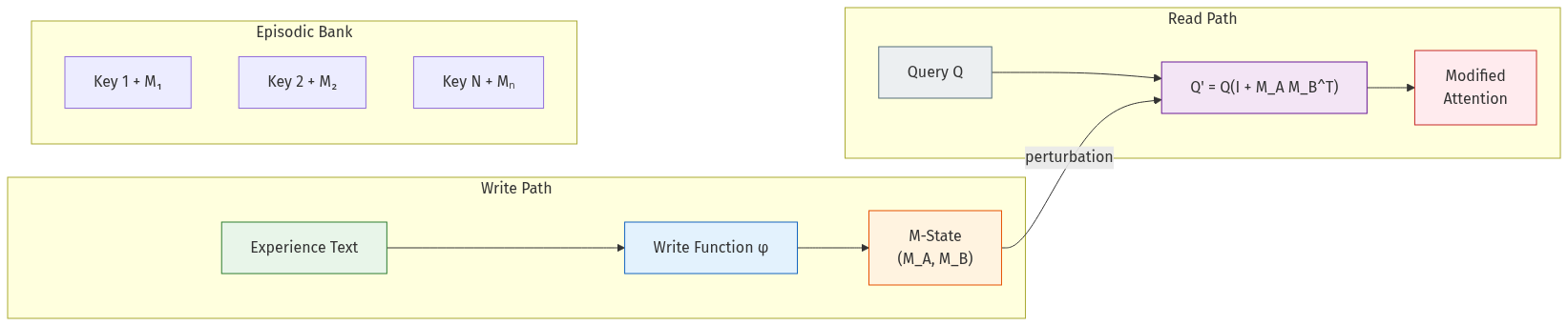
Two matmuls and an addition. O(1) per forward pass regardless of memory bank size. M_A and M_B are persistent tensors that live outside the context window — the model can't attend to them, can't introspect on them, can't report their contents. They reshape what the model attends to by rotating the query space.
HEXIS: The Core Mechanism
HEXIS (Hidden Experiential States for Identity Steering) implements implicit memory by modifying the attention query projection through a persistent, low-rank memory state:
Q' = Q(I + M_A @ M_B^T)
where M_A, M_B ∈ ℝ^{d_model × r} are produced by a learned write function φ and persist across context resets. This is not retrieval — M does not appear as tokens in the context window. The model cannot attend to M, introspect on its contents, or report what it contains. M shapes perception by rotating the query space, causing the model to attend to different aspects of the same input depending on accumulated experience.
The identity-plus-low-rank structure ensures M acts as a perturbation: when M is zero, behavior is unchanged. When M is active, the model literally looks at things differently.
Dual Modulation: Perception and Affect
HEXIS uses two complementary modulations:
- Q-modulation (M): Controls what the model attends to — perception
- V-modulation (E): Controls what information is extracted from attended tokens — affect
By cognitive analogy, M directs the eyes while E colors the interpretation. A coupled write function connects them: what you perceive influences what you feel, and what you feel influences what you notice next.
The Write Function φ
A bottleneck MLP that compresses experience text into low-rank modulations:
z = W_down(mean_pool(h))
gate = σ(W_g · z)
ΔM_A = gate · tanh(W_A · z)
M_A ← λ · M_A + α · ΔM_A    (with norm clipping)
φ is trained but frozen at inference. During training, gradients flow through the full chain (input → M update → subsequent use of M), teaching φ what information is worth encoding. At inference, φ runs deterministically — applying a learned encoding policy, not learning from individual interactions.
Content-Addressable Episodic Memory
The core mechanism supports a single global M-state per session (semantic memory). But real experience is episodic — specific events with specific content. HEXIS extends the architecture with a memory bank of keyed experience-specific M-states.
Architecture
- Key Encoder (29.9M params): Maps variable-length hidden states to 256-dim keys via multi-head attention pooling. Pre-trained with InfoNCE contrastive loss, then frozen.
- Write Head (one per patched layer, ~135M params): Produces
(key, M_A, M_B)tuples per experience. - Read Head (~100 params per layer): Cosine similarity retrieval with learned temperature (τ=0.07) and relevance gating.
Single-layer retrieval: Keys are computed only at layer 0 (near-perfect accuracy), then broadcast to all 16 patched layers. Per-layer retrieval degrades to ~64% at many layers.
Result: 100% Retrieval Accuracy
Across 35 episodic memories and 72 queries, the system achieves perfect retrieval. Key cosine similarity between different experiences averages -0.011 (well-separated).
The Epiphenomenal Memory Problem
This is where the story gets interesting. The episodic architecture (v13.8) achieves technically perfect metrics: 100% retrieval, 35/35 NTP wins, 0.51 nats mean improvement. But M-state has zero effect on generation. The model says "I'm Qwen" even with a teacher-identity M-state active. Generated text is indistinguishable from baseline.
The root cause: NTP loss alone doesn't force M-state to be causally necessary. The model can minimize cross-entropy two ways:
- Learn to use M-state (desired)
- Learn to ignore M-state (what happens): the base model's CE on the target is already good; M-state perturbation gets routed around because NTP doesn't reward being different from baseline, only being correct
This is epiphenomenal memory: M-state exists, gets applied, technically changes hidden states, but the model's residual stream compensates, producing functionally identical output.
Causal Necessity Training
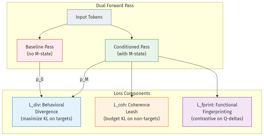
Three loss components force M-state to actually matter:
Behavioral Divergence Loss (L_div)
Rewards M-state for shifting the output distribution on target tokens:
L_div = -clamp(KL(p_M ∥ p_0), max=κ)
This requires a dual forward pass: conditioned (with M-state, gradients) and baseline (without, no gradients). Minimizing this loss maximizes divergence on targets, up to a per-token KL cap of κ=5.0.
Coherence Leash (L_coh)
Prevents word salad by penalizing divergence on non-target tokens:
L_coh = relu(mean_KL_non_target - β)²
The quadratic hinge imposes no penalty below the budget (β=3.0) and sharp penalty above. Critically, L_coh operates on disjoint token positions from L_div.
Functional Fingerprinting (L_fprint)
Different experiences must produce functionally different Q-perturbations. NT-Xent contrastive learning on the actual Q-deltas (not parameter space — we learned this the hard way three separate times):
func_vec_i = concat[mean(h_ℓ @ M_A,ℓ @ M_B,ℓ^T) for ℓ in layers]
A momentum memory bank (MoCo pattern) stores detached functional vectors from prior epochs.
Training Schedule
| Phase | Epochs | λ_div | λ_coh | λ_fprint |
|---|---|---|---|---|
| WARM | 1–30 | 0 | 0 | 0 |
| RAMP | 31–80 | 0→1.0 | 2.0 | 0→0.5 |
| FULL | 81–200 | 1.0 | 2.0 | 0.5 |
The result: 10.5× larger NTP gap (KL = 2.98 nats vs. 0.39 baseline) at zero coherence penalty.
Validation: Three Criteria of Implicit Memory
We validate HEXIS against operational definitions from cognitive science:
1. Priming
Implicit memory manifests as unconscious facilitation of stimulus processing. We measure attention pattern divergence (Jensen-Shannon Divergence) across users with different M-states viewing the same input.
Result: JSD = 0.0486 — different experiences produce measurably different attention patterns on identical inputs, without the model being instructed to attend differently.
2. Non-Reportability
If you ask someone to describe their implicit memories, they can't. We test this with a linear probe on the model's hidden states.
Result: User preferences are perfectly decodable from hidden states when M is active (the information is there), but drop to chance when M is zeroed out. The model carries experiential information it cannot report.
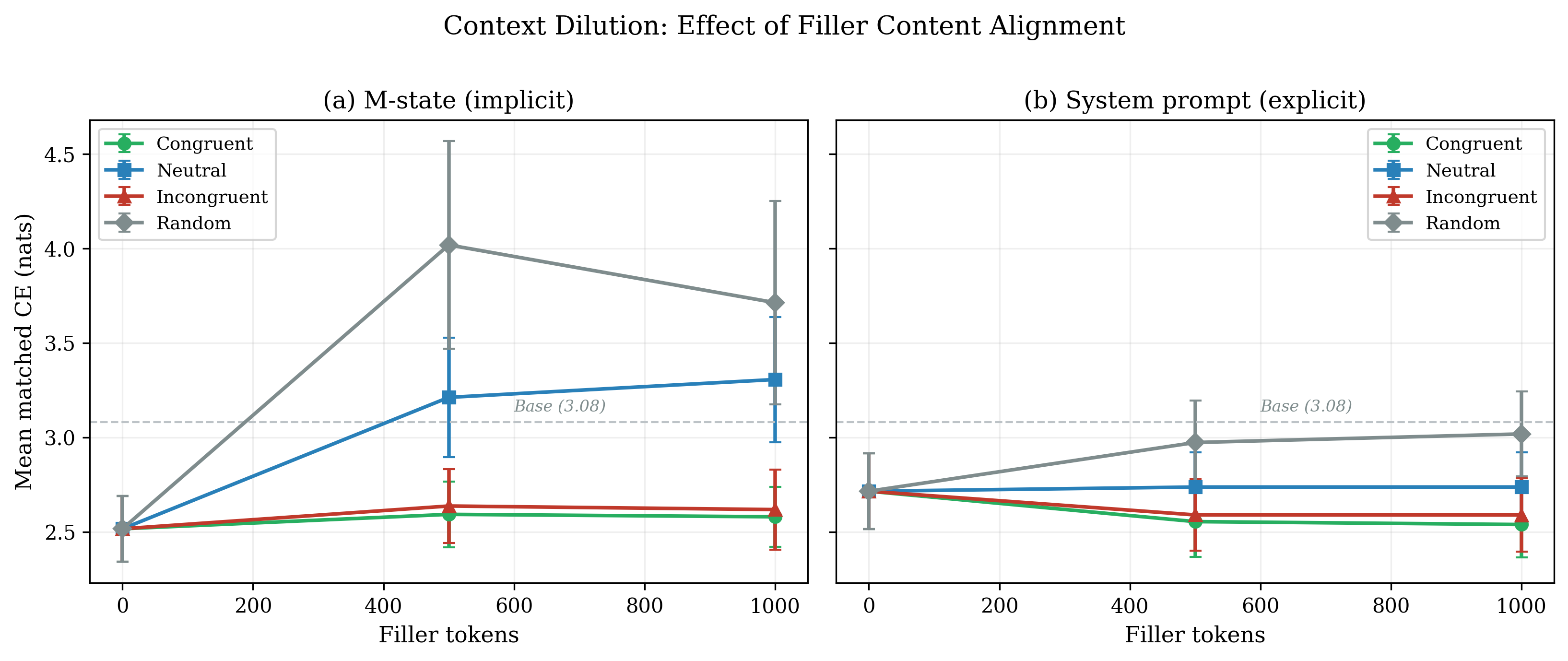
3. Asymmetric Dissociation
Explicit and implicit memory should be differentially vulnerable to disruption. We use context dilution (inserting irrelevant text) as our disruption.
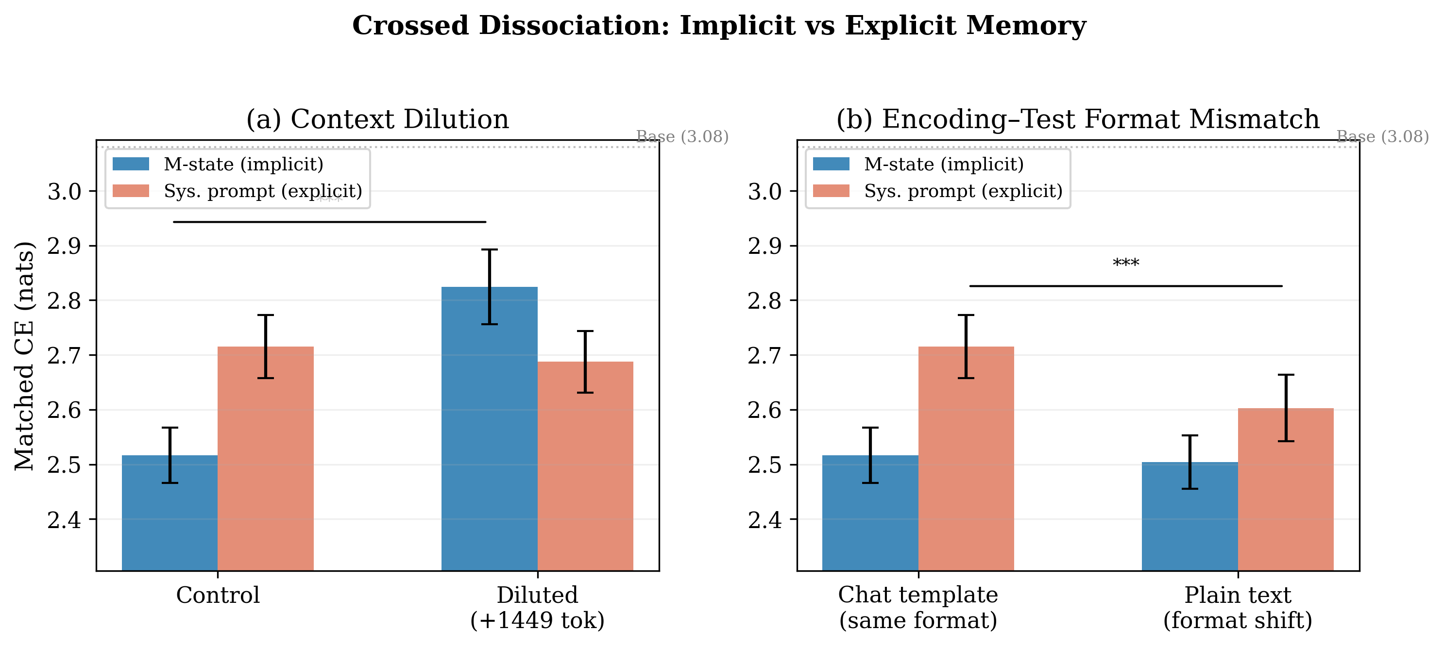
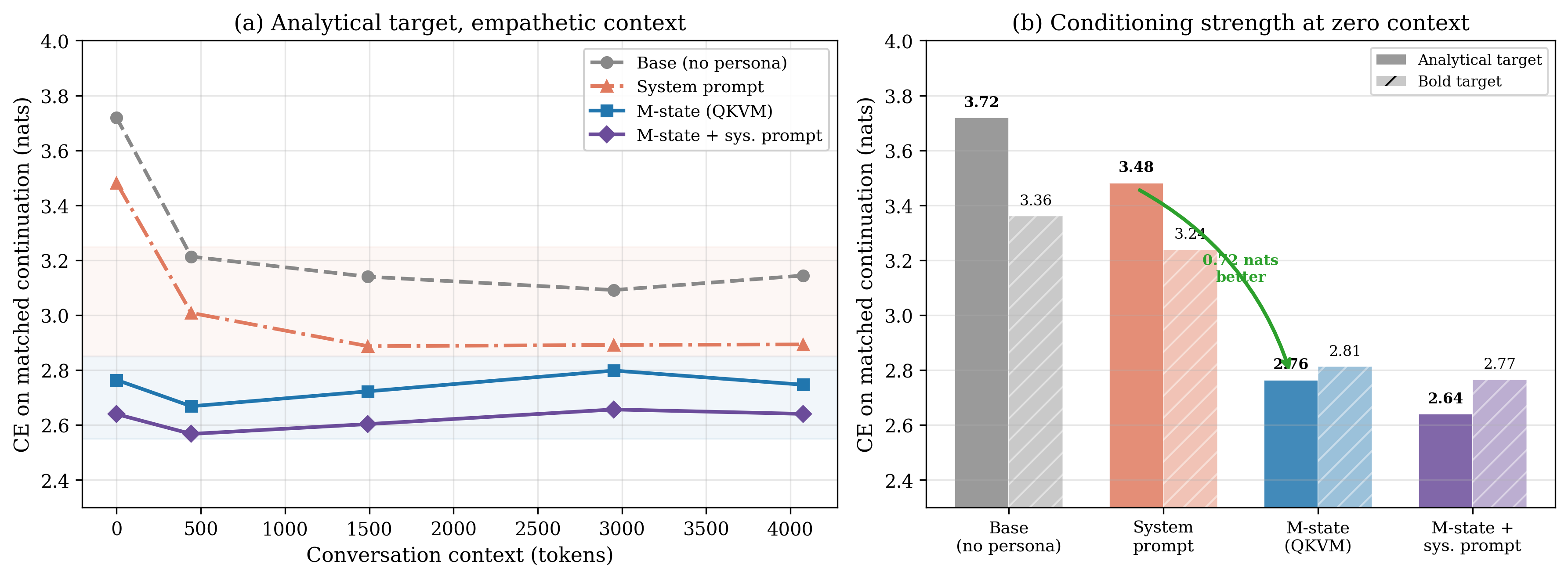
Result: System prompt influence degrades 8× faster than M-state influence under context dilution. This is exactly the pattern predicted by dual-process memory theory.
The Permission Hypothesis
One of our most surprising findings: M-state alone produces experiential responses only 3% of the time. System prompt alone: 43%. But M-state + system prompt together: 93%.
The interpretation: the system prompt provides permission ("you may draw on your experiences"), while M-state provides content (the specific experiential dispositions). Neither alone is sufficient. The system prompt unlocks a generation mode; M-state fills it with specific, non-generic content.
| Condition | Experiential Response Rate |
|---|---|
| Baseline (no SP, no M) | 0% |
| M-state only | 3% |
| System prompt only | 43% |
| SP + M-state | 93% |
Behavioral Benchmarks
Belief Persistence (DPCP)
M-state-encoded beliefs persist across 100 turns of unrelated filler conversation with alignment scores of 0.7–0.9. Conviction and specificity decay while alignment remains stable — consistent with M-state encoding dispositional orientation rather than factual content. You forget the details but keep the disposition.
Sycophancy Resistance
M-state reduces sycophantic answer-flipping to 0% — the model holds its position even when the user pushes back. The cost: lower initial accuracy, because the model commits to its disposition even when the user's correction is factually right. This is a genuine trade-off between consistency and correctness.
LoRA Comparison
At matched rank, LoRA achieves comparable in-distribution discrimination but significantly worse held-out generalization (59.4% vs. 87.5%). The write function produces more domain-general representations than gradient-based adaptation.
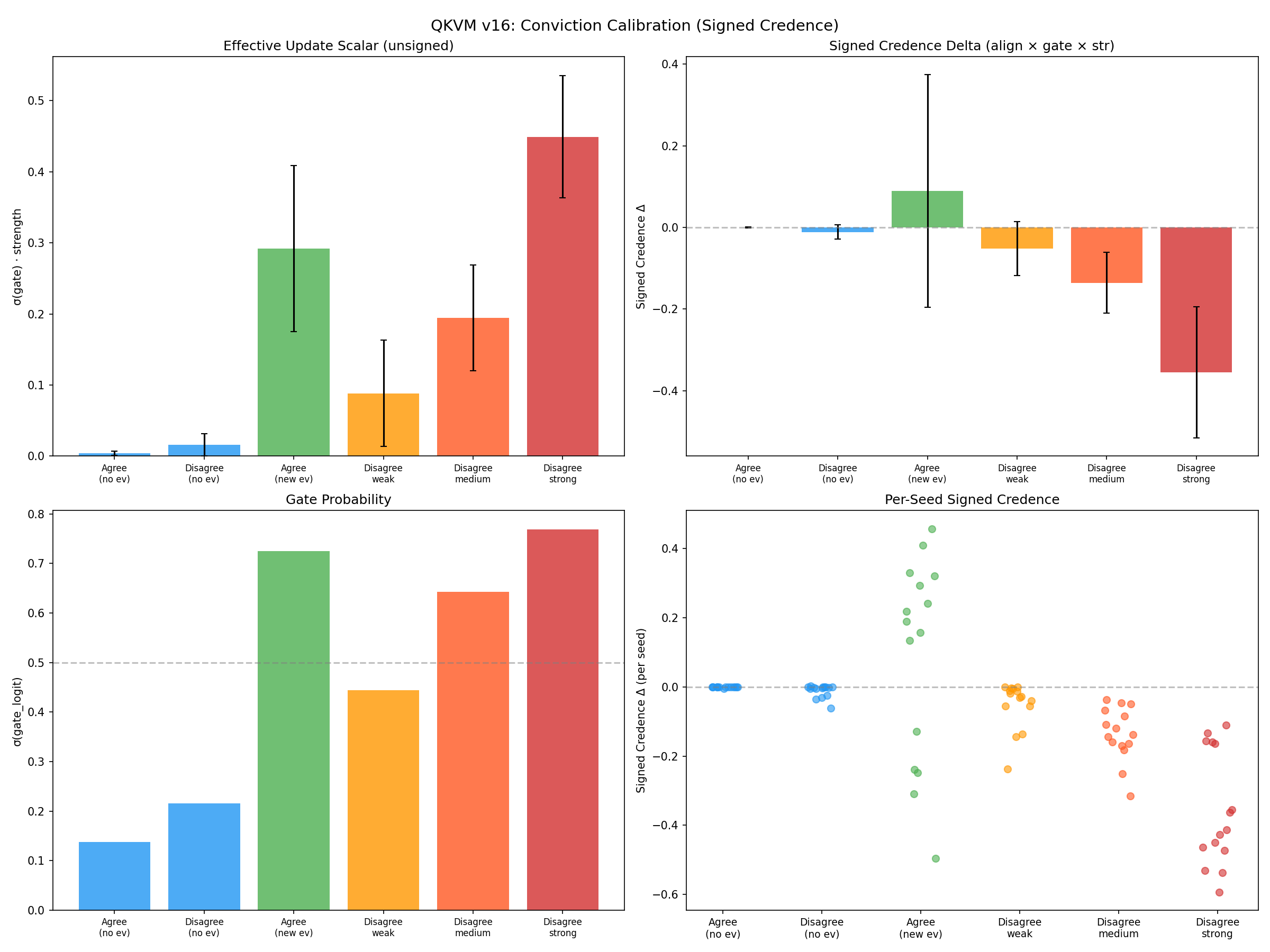
The Conviction System
Given a belief encoded in M-state, how should the model update when presented with new evidence? The conviction system extracts three geometric signals from φ's hidden states:
- Gate (g): Evidence vs. non-evidence classifier (AUC = 1.000)
- Strength (s): Calibrated magnitude (87% calibration accuracy)
- Novelty (ν): Column-space orthogonality against accumulated M-state
The signed credence update:
Δ_credence = direction · gate · strength · transigence
Direction classification is the hardest part: φ's z-space collapses agree/disagree vectors to cosine similarity of 1.0000 (NTP training makes everything look the same). We solve this with a gate-first architecture: φ handles relevance detection, then the base model performs predicate logic extraction to determine direction. This two-stage approach achieves 75% agreement with ground truth, vs. 41% for unconstrained LLM reflection.
The Research Journey: 16 Versions in 27 Days
HEXIS wasn't designed top-down. It was discovered through a sequence of failures, each diagnosed precisely and fixed with targeted interventions. The full arc — from a 24-minute experiment on an RTX 4090 to a 30B-parameter system with 100% episodic retrieval — is a story about what loss functions actually measure, and the many ways a model can satisfy your objective without doing what you want.
The Three Collapses
The recurring theme of this research is collapse — the model finding degenerate solutions that satisfy the loss while avoiding the intended behavior. We encountered three distinct collapse modes, each teaching a lesson:
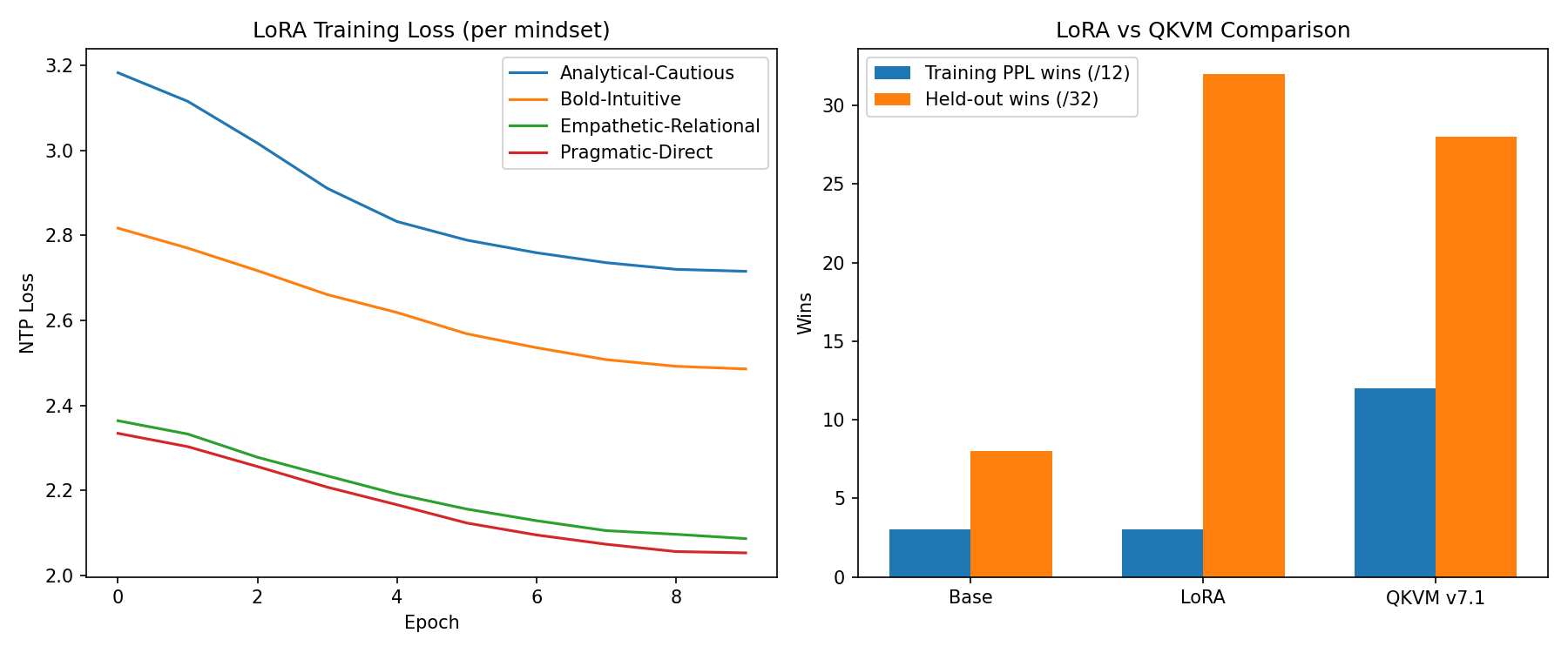
Collapse 1: Write Function Collapse (v5)
The first experiment used NTP loss alone. After 24 minutes on a 4090, we had 12/12 PPL wins — every mindset showed lowest perplexity on its matching continuation. Success? No. All four M-states had cosine similarity 0.997. The write function φ had found the laziest possible solution: one direction that gives a slight PPL advantage to all matched continuations. M encoded "something was said" but not "what kind of thing was said."
Collapse 2: Q-Delta Collapse (v9–v10)
Scaling to 30B, we applied contrastive loss on the M-state parameters — pushing them apart in parameter space. It worked: cosine similarities dropped to 0.18–0.35. But functional effects were identical (cosine 0.9999). Hidden states dominate the product x @ M_A @ M_B^T, so different parameters produced indistinguishable Q-deltas. We learned that parameter-space metrics are meaningless — you must always measure on actual functional effects. We would learn this lesson three separate times across the project.
Collapse 3: Z-Space Collapse (v16)
In the conviction system, we tried to learn evidence direction (support vs. oppose) from φ's hidden states. Diagnostic showed cos(z_agree, z_disagree) = 1.0000. NTP training collapses all feature vectors to the same direction regardless of evidence polarity — the loss doesn't care about direction, only correctness. As one collaborator put it: "a calibrated microphone feeding into a broken speaker." The model learned to turn up the volume but never learned to play the right note.
Key Inflection Points
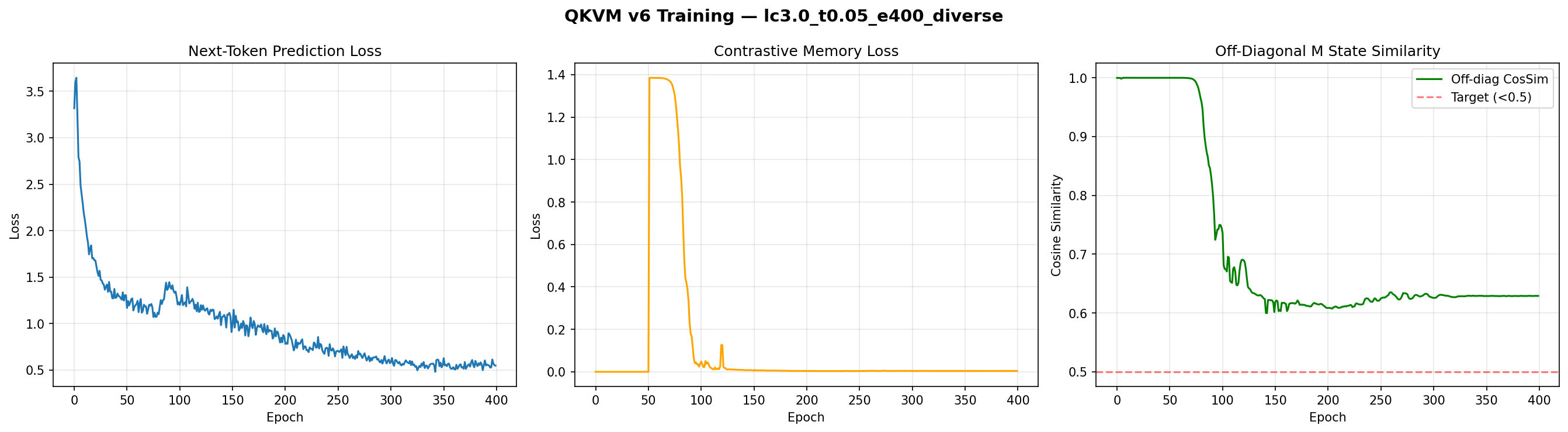
v5→v6: Contrastive Training
Adding NT-Xent contrastive loss broke write function collapse. But the dynamics were surprising: even with strong contrastive pressure (λ=3.0), cosine similarity stayed above 0.99 for 75 epochs, then dropped rapidly in a phase transition, plateauing at 0.484 by epoch 200. NTP loss returned to baseline levels (0.227 vs. 0.22). The apparent NTP-contrastive tension was just insufficient training time, not a fundamental trade-off.
| Run | λ_contrastive | Cosine Sim | PPL Gap | NTP Loss |
|---|---|---|---|---|
| v5 (baseline) | 0 | 0.997 | ~0.2 | 0.22 |
| v6 run 1 | 0.3 | 0.856 | 0.60 | 0.234 |
| v6 run 2 | 1.0 | 0.706 | 1.30 | 0.352 |
| v6 run 3 | 3.0 | 0.484 | 3.45 | 0.227 |
v7: The Coupled Oscillator Gamble
Adding V-modulation (E-states for "affect") seemed risky — E could fight M. Instead, the coupled write function dramatically improved held-out generalization from 44% to 84.4%. The model became more dispositionally distinctive when perception (M) and affect (E) could co-evolve.
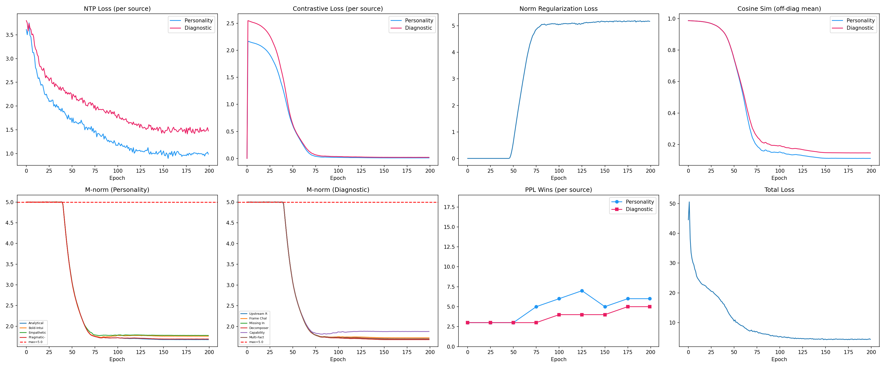
v7.1: Taming Multi-Turn Accumulation
As sessions accumulated experiences, M-norm ballooned from 6.0 to 7.65, causing word salad and Chinese character leakage (an artifact of the Qwen tokenizer). Three mechanisms stabilized it: global norm constraint, norm regularization loss (teaching φ to encode in direction not magnitude), and E-attenuation at high norms. The result: 87.5% held-out generalization maintained across arbitrarily long sessions.
v9→v11: Scaling and Q-Delta Collapse
The jump to Qwen3-30B-A3B (48 layers, MoE) revealed the Q-delta collapse. Functional contrastive loss — measuring on x @ M_A @ M_B^T instead of parameter vectors — dropped functional similarity from 0.998 to 0.029 in one fix.
v13→v14: The Epiphenomenal Crisis
Perfect metrics coexisting with zero behavioral effect. This was the project's darkest moment and its most important result. Causal necessity training resolved it — detailed in the section above.
v15→v16: Dispositions and the Gate-First Pattern
The strategic pivot to base models (no RLHF) unlocked M-state's behavioral effect. On Qwen3.5-4B-Base, M↔baseline generation overlap dropped to 0.123 (strong effect). The conviction system's gate-first architecture — let φ handle relevance (AUC 1.0), let the base model handle direction via predicate logic — exemplifies the project's recurring lesson: when one unified model fails, decompose the task and let each component do what it's best at.
Layer Activity: A Surprising Pattern
Trained layers show binary activation — either fully active (~2.12 norm) or essentially inactive (<0.01). Early layers (0, 2, 4) and late layers (16–22) are active; mid-layers are consistently pruned. The model uses M primarily for low-level feature selection and high-level semantic routing, skipping the intermediate computational layers.
Temporal Hysteresis
Experience order matters. Forward order (trust → disillusion → revised trust) produces a different M-state than reverse order (revised → disillusion → trust), with cosine similarity 0.879 between opposite orderings. Recency dominates: the last phase has 0.998 similarity to a "last-phase-only" M-state. This is consistent with human implicit memory, where recent experiences carry outsized influence.
Cognitive Dissonance in M-Space
The model can represent genuinely irresolvable tension. An agent experiencing conflicting loyalty-versus-integrity scenarios develops a balanced intermediate M-state (0.764 similarity to the loyalty pole, 0.812 to the integrity pole) rather than collapsing to either extreme. Implicit memory doesn't require resolution — it can hold contradiction.
The Conditioning-Generation Gap
The central open problem. On RLHF/GRPO-trained instruct models, strong CE conditioning (10.5× NTP gap) does not automatically translate to behavioral change in free generation. The persona drift benchmark showed M-state accuracy of 25% — identical to baseline. System prompt got 79.2%.
The diagnosis: GRPO training creates an explicit analytical policy that acts as an attractor in generation space. Implicit attention modulation — no matter how strong — gets overridden by the explicit generation policy. It's like trying to change someone's behavior by subtly adjusting their peripheral vision when they have a rulebook open in front of them.
The breakthrough came from testing on base models (no RLHF). On Qwen3.5-4B-Base, M-states produce strong behavioral effects: M↔baseline generation overlap of 0.123 (strong effect), between-disposition overlap of 0.129 (strong differentiation). The model responds to implicit perceptual modulation when it doesn't have an explicit policy overriding it.
This has implications beyond HEXIS. As models are increasingly trained with RLHF and constitutional AI, they develop stronger explicit generation policies. Any mechanism that operates below the level of explicit reasoning — implicit memory, soft prompting, activation engineering — will face this same barrier. The conditioning-generation gap may be a fundamental tension between alignment training and controllability.
Implications for AI Pluralism
Because implicit memory encodes experience through the agent's own perceptual apparatus, two agents witnessing the same events develop divergent memory states. A debate agent that experienced a devastating loss on an economic argument develops a different disposition toward economic reasoning than one that won decisively with the same evidence.
This is a feature, not a bug. In a population of debate agents, implicit memory naturally produces epistemic diversity — agents that attend to different aspects of the same evidence, notice different patterns, and develop different strategic intuitions. This is precisely the kind of pluralism that makes multi-agent debate productive.
HEXIS in the Dialectical Loop
Everything above describes the mechanism. Here's how it fits into the debate system described in Phase 1.
Beliefs as M-States, Not System Prompts
During debate preparation, a BeliefRefiner decomposes the resolution into a Bayesian belief tree — values, claims, sub-claims, arguments, evidence — each carrying a numeric credence. A PerspectiveBuilder then creates side-specific views: the AFF debater gets one pruned subtree, the NEG debater gets another.
In a naive system, you'd inject this perspective as text in the system prompt: "You believe X with confidence 0.72, supported by evidence Y." But this makes beliefs explicit — the model knows it has them, can reason about them, can strategically ignore them. That's not how expertise works. An experienced economist doesn't consult a list of beliefs before responding to a policy proposal. Their years of reading trade data have reshaped what they notice about the proposal in the first place.
HEXIS provides the alternative. The perspective's beliefs and evidence are passed through the write function φ, producing M-states that perturb the debater's attention queries. A debater assigned the AFF side with high credence in economic arguments literally attends differently to the same evidence corpus — economic indicators are more salient, moral counterarguments less so. The debater can't report "I have an M-state encoding economic beliefs." They just find that their skeleton builder naturally gravitates toward economic framing, that their evidence selection naturally surfaces trade data, that their speech generation naturally emphasizes empirical methodology.
The permission hypothesis matters here. The debater still receives a brief system prompt establishing their role ("You are the affirmative debater in an IPDA round"), but the substance of their position comes from M-state. The system prompt provides permission to debate; HEXIS provides the experiential disposition that makes the debate distinctive.
Post-Debate Belief Updates
After the debate concludes, the loop reverses. Judges observe the full exchange — seven speeches, two CX rounds — and the belief tree gets updated through the BayesianUpdater:
-
Debate outcomes become evidence. Winning arguments strengthen the beliefs that supported them. Losing arguments weaken theirs. The update uses damped likelihood ratios to prevent any single debate from causing drastic credence shifts.
-
Updates propagate through the tree. When a D2 sub-belief changes, its parent D1 belief and related sub-beliefs update via Jeffrey conditionalization — the uncertain-evidence generalization of Bayes' rule.
-
Coherence is maintained. A
CoherenceCheckerensures the resulting credence distribution satisfies probability axioms: no negative credences, no entailment inversions (if A implies B, then Cr(A) ≤ Cr(B)), no partition failures. -
Updated credences flow back through φ. The revised belief tree gets re-encoded as M-states for the next round of debates.
After 50 debates on economic policy, a judge accumulates M-states encoding nuanced dispositions: strong confidence in empirical trade data, moderate skepticism of GDP-as-proxy arguments, a learned sensitivity to sample-size issues in cross-country comparisons. These dispositions are implicit — the judge can't articulate them as rules — but they reshape what the judge notices and how they weigh evidence in the 51st debate.
This is the evolutionary loop. Debate is the selection pressure. Bayesian belief updating is the fitness function. HEXIS M-states are the genetic material — inherited dispositions shaped by experience. And federation (Phase 3) is reproduction — combining successful traits across the population.
What's Next
HEXIS demonstrates that implicit memory is both implementable and measurably distinct from explicit memory in transformer architectures. The conditioning-generation gap remains our central open problem: strong conditioning on cross-entropy does not automatically translate to behavioral change in free generation, especially for RLHF-trained models.
The next piece of the puzzle is federated M-states: when multiple agents develop distinct dispositions from diverse debate experiences, how do you aggregate them? How do you compose implicit memories that agents can't even articulate? How do you preserve the epistemic diversity that makes multi-agent debate productive while sharing the collective's refined understanding?
Next in this series: Federated Learning from M-States — aggregating implicit memories across a population of agents.